Deriving the Speed of Light

I honestly don’t know where to start writing this, but from now on I’m going to write down everything I’ve learned so I don’t forget it. Writing helps strengthen memory and moves information from short-term memory to long-term memory. So, I hope starting from now I’ll be consistent with writing. Whether I’ll publish it to a blog, or just keep it in Obsidian, haha, we’ll see. I started writing this on April 15th and I’ll be adding to it gradually, whenever I’m in the mood to write.

The triangle formula $V = I \cdot R$ (Ohm’s Law) is super important for engineers, especially in electrical and electronics engineering, because it’s the fundamental foundation for understanding, designing, and analyzing electrical circuits. But this time, we’re going to talk about the most fundamental reason in the universe for why electricity ($I$) and voltage ($V$) can even exist and interact with each other, through the 4 Maxwell’s Equations. We’ll be focusing on the 3rd and 4th equations, because that’s what will bring us to the topic in our title. Through these equations, we can also understand why we’re able to enjoy WiFi signals, radio, and all that good stuff today. I’ll try to explain it slowly and in detail while also trying to keep the language easy to understand (I hope so, haha). So don’t panic yet when you see the intimidating numbers and symbols.

The Four Maxwell’s Equations

Long before Maxwell unified electricity and magnetism, physicists had already measured two intrinsic properties of the universe (specifically, of a vacuum). The main concept we need to hold onto at this stage is: The vacuum of our universe (like the empty void of outer space) is NOT a place that is truly “empty” or “dead”. A vacuum is more like a canvas. This canvas has built-in properties, namely how flexible it is in allowing “electricity” and “magnetism” to exist within it. These built-in properties are what get measured by those two constant numbers.

Let’s break them down one by one:

a. Permittivity of Free Space ($\epsilon_0$)

• This is the number that shows how “supportive” a vacuum is in allowing an electric field to form.
• Its unit (Farads per meter - $\text{F/m}$):
  • Farad (F) is the unit for Capacitance (the ability to hold and store electrical energy). We’re definitely familiar with a device called a “capacitor” or a battery. Their power to store electricity is measured in Farads. 1 Farad is actually a massive amount of storage capacity.
  • per meter (m) means we’re measuring this electricity-storing ability for every 1 meter of distance in a vacuum.
• What’s the value?: It’s $\approx 8.854 \times 10^{-12} \, \text{F/m}$. Written out normally, that’s 0.000000000008854 F/m.
• What it means: This number is incredibly small. It means a vacuum is actually pretty “stiff” and poor at holding pure electricity compared to other materials (like glass or plastic). But even though it’s small, that electrical property is still there in empty space.

b. Permeability of Free Space ($\mu_0$)

• This is the opposite. It’s the number that shows how “supportive” a vacuum is in allowing a magnetic field to penetrate and form within it.
• Its unit (Henries per meter - $\text{H/m}$):
  • Henry (H) is the unit for Inductance. Inductance is simply the “magnetic pull and push effect” that happens when there’s a fluctuating flow of electricity.
  • per meter (m) means the ability to create this magnetic effect is measured per every 1 meter.
• What’s the value?: It’s exactly $4\pi \times 10^{-7} \, \text{H/m}$, or roughly 0.000001256 H/m.
• What it means: Again, the number is incredibly small. A vacuum doesn’t have any metallic material (like iron) in it, so it’s very weak at supporting the formation of a magnetic field, but its ability is not zero.

These two constants are quietly hidden inside Maxwell’s 4th equation. And as we’ll see later, when Maxwell started tinkering with the 3rd and 4th equations mathematically, these two tiny numbers suddenly revealed something he never expected. Yep, the speed of light! But before that, let’s get familiar with the 4 Maxwell’s Equations below:

a. Gauss’s Law for Electricity

$$\nabla \cdot \mathbf{E} = 0$$

• What it means: In a vacuum, there is no electric field ($\mathbf{E}$) radiating outward from any point.
• Why is it 0?: Because electric fields originate from charges (like protons or electrons). Since we’re in a completely empty space with no charges, the radiation is zero.

b. Gauss’s Law for Magnetism

$$\nabla \cdot \mathbf{B} = 0$$

• What it means: The magnetic field ($\mathbf{B}$) never radiates straight outward from a single point.
• Why is it 0?: Because in the universe, a single magnetic charge (just a North pole or just a South pole on its own) simply does not exist. Magnetic field lines always curve and loop back from North to South. They never just shoot off freely in one direction.

c. Faraday’s Law

$$\nabla \times \mathbf{E} = -\frac{\partial \mathbf{B}}{\partial t}$$

• What it means: A swirling electric field ($\nabla \times \mathbf{E}$) is created whenever there’s a change in the magnetic field over time ($\frac{\partial \mathbf{B}}{\partial t}$).
• Note: The minus sign ($-$) there comes from Lenz’s Law, which means this swirling effect will always “oppose” whatever caused the change in the first place.

d. The Ampere-Maxwell Law

$$\nabla \times \mathbf{B} = \mu_0 \epsilon_0 \frac{\partial \mathbf{E}}{\partial t}$$

• What it means: A swirling magnetic field ($\nabla \times \mathbf{B}$) is created whenever there’s a change in the electric field over time ($\frac{\partial \mathbf{E}}{\partial t}$).
• Note: This is where our two constants ($\mu_0$ and $\epsilon_0$) finally show up! They act as a multiplying bridge that determines how large of a magnetic field gets created from a changing electric field in a vacuum.

Take a look at the 3rd and 4th equations! They influence each other, right? This is where things get really interesting. If a magnetic field starts vibrating and changing, it creates an electric field (Equation 3). Because this newly born electric field is also vibrating and changing, it automatically creates a brand new magnetic field (Equation 4). That new magnetic field creates another electric field, and so on and so on!

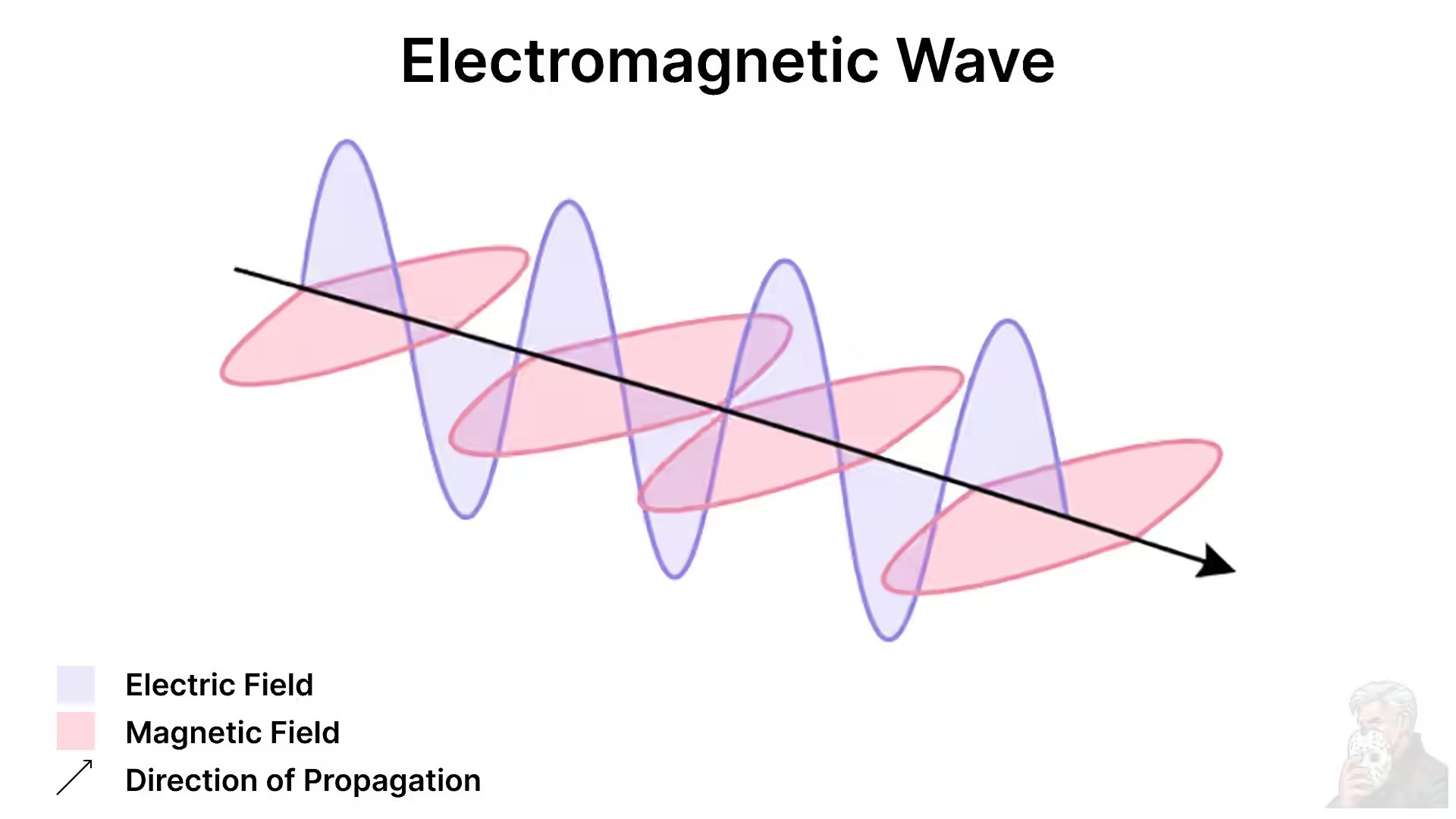
The two of them mutually support each other, mutually create each other, and dance together through the vacuum without needing any medium at all. Maxwell realized something was dancing out there. This traveling “dance” is what we call Electromagnetic Waves, which in their real form we experience every single day as sunlight, WiFi signals, radio waves, and X-rays.

From this, Maxwell was able to “predict” the speed of light through pure math alone, because his equations concluded that electromagnetic waves travel at the speed of light. Haha, honestly when I found this out I was absolutely in awe of how brilliant the scientists of the past were. Maxwell formulated his equations, and then Hertz, a few years after Maxwell’s death, experimentally proved that electromagnetic waves actually exist by creating and detecting radio waves for the very first time (what we now know as Radio Waves). Pretty cool right? Okay, now that we understand the “phenomenon”, let’s dig into the math.

Derivation of the Speed of Light from Maxwell’s Equations

We’re going to use vector calculus, determinant matrices, and linear algebra to work through this.

Faraday’s Law

Let’s break down Faraday’s Law first.

$$\nabla \times \mathbf{E} = -\frac{\partial \mathbf{B}}{\partial t}$$

The right side shows the change in the magnetic field, and the left side shows the swirling electric field that always accompanies it. More precisely, both happen simultaneously. This is a correlation, not a pure cause-and-effect. But to get the intuition, we can read it as: a changing magnetic field “brings forth” an electric field.

We’re going to simplify this from three dimensions down to one dimension, starting from the left side, $\nabla \times \mathbf{E}$.

Part 1

We’re going to agree that electricity vibrates up and down in this setup. But first, let’s recall these three things:

• $x$-axis (horizontal): $\hat{i}$
• $y$-axis (vertical/up-down): $\hat{j}$
• $z$-axis (depth/forward-backward): $\hat{k}$

We already agreed at the start: to make the wave easy to calculate (1 Dimension), we set it up so that the Electric Field wave ($\mathbf{E}$) purely vibrates up and down. Now let’s translate the words “up and down” into the language of those 3 compass directions.

Try raising your right hand right now, then shape your fingers like a gun with your middle finger bent 90 degrees toward you:

• Thumb ($x$-axis / $\hat{i}$ direction): Points straight to the right.
• Index finger ($y$-axis / $\hat{j}$ direction): Points straight up.
• Middle finger ($z$-axis / $\hat{k}$ direction): Points toward your own face.

Part 2

Up and down is the path of your index finger, which is the $y$-axis. Its compass is $\hat{j}$. It does not vibrate along the thumb direction ($x$-axis / $\hat{i}$). It does not vibrate along the middle finger direction ($z$-axis / $\hat{k}$).

So, if we want to write the complete form of the Electric Field ($\mathbf{E}$) in this story mathematically, we need to check it against all three axes:

• $x$ direction: $0\hat{i}$
• $y$ direction: $E_y\hat{j}$ (we name it $E_y$ so we remember this is the Electric value on the $y$-axis)
• $z$ direction: $0\hat{k}$

Combining everything into one line, the mathematical identity of our Electric Field ($\mathbf{E}$) is now officially written as: $$\mathbf{E} = 0\hat{i} + E_y\hat{j} + 0\hat{k}$$

Part 3

Try to recall the shape of Faraday’s Law from earlier: there’s a symbol that looks like an upside-down triangle ($\nabla$). That symbol is called Nabla.

In the world of calculus, Nabla is like a 3-Dimensional scanner or sensor tool. It has one job: detecting whether there is any “change” around it.

Just like how we broke the Electric Field ($\mathbf{E}$) in Part 2 into 3 compass directions, this Nabla machine also has 3 “sensors” for detecting change along all three axes:

• Sensor $x$ (forward/backward): $\frac{\partial}{\partial x}\hat{i}$
• Sensor $y$ (up/down): $\frac{\partial}{\partial y}\hat{j}$
• Sensor $z$ (left/right): $\frac{\partial}{\partial z}\hat{k}$

If we combine all three sensors of the Nabla machine into one line (just like how we wrote the Electric Field earlier), its official identity is written as:

$$\nabla = \frac{\partial}{\partial x}\hat{i} + \frac{\partial}{\partial y}\hat{j} + \frac{\partial}{\partial z}\hat{k}$$

Now with all three of those in hand, let’s put them together into a cross product table (a matrix).

Part 4

We have the Nabla machine ($\nabla$) from Part 3, and we have the Electric Field form ($\mathbf{E}$) from Part 2. Between them sits a cross/curl sign ($\times$), which means we’re doing a Cross Product operation (Vector Cross Multiplication).

In calculus, the way to compute a Cross Product is by stacking all of our ingredients into a 3-floor table (3x3 Matrix). The rules for arranging each floor are strict and cannot be swapped around:

• Floor 1 (Top): Always filled with the 3 compass direction pointers ($\hat{i}, \hat{j}, \hat{k}$).
• Floor 2 (Middle): Always filled with the change sensors from the Nabla machine ($\frac{\partial}{\partial x}, \frac{\partial}{\partial y}, \frac{\partial}{\partial z}$).
• Floor 3 (Bottom): Always filled with the Electric Field values from Part 2 ($0, E_y, 0$).

If we arrange everything neatly, the official mathematical form becomes:

$$\nabla \times \mathbf{E} = \begin{vmatrix} \hat{i} & \hat{j} & \hat{k} \\ \frac{\partial}{\partial x} & \frac{\partial}{\partial y} & \frac{\partial}{\partial z} \\ 0 & E_y & 0 \end{vmatrix}$$

Part 5

Now let’s compute this using the matrix determinant.

$$\begin{vmatrix} \hat{i} & \hat{j} & \hat{k} \\ \frac{\partial}{\partial x} & \frac{\partial}{\partial y} & \frac{\partial}{\partial z} \\ 0 & E_y & 0 \end{vmatrix}$$

In our Floor 1, the letters $A$, $B$, and $C$ are now replaced by the compass direction pointers $\hat{i}$, $\hat{j}$, and $\hat{k}$. Let’s break this big table into three $2 \times 2$ boxes using the Cofactor Expansion Method.

1. Focus on $\hat{i}$ (Positive)

Cover the top row and left column.

$$+\hat{i} \begin{vmatrix} \frac{\partial}{\partial y} & \frac{\partial}{\partial z} \\ E_y & 0 \end{vmatrix}$$

2. Focus on $\hat{j}$ (Negative)

Cover the top row and middle column.

$$-\hat{j} \begin{vmatrix} \frac{\partial}{\partial x} & \frac{\partial}{\partial z} \\ 0 & 0 \end{vmatrix}$$

3. Focus on $\hat{k}$ (Positive)

Cover the top row and right column.

$$+\hat{k} \begin{vmatrix} \frac{\partial}{\partial x} & \frac{\partial}{\partial y} \\ 0 & E_y \end{vmatrix}$$

Now let’s “cross multiply and subtract” to solve each box:

• Box $\hat{i}$:
  • First cross: $\frac{\partial}{\partial y} \times 0 = 0$.
  • Second cross: $\frac{\partial}{\partial z} \times E_y = 0$ (Because our wave only travels forward along the $x$-axis, so the $z$-axis sensor detects no change whatsoever. The wave only propagates along the x-axis, not the z-axis.)
  • Final result: $0 - 0 = \mathbf{0}$.
• Box $\hat{j}$:
  • First cross: $\frac{\partial}{\partial x} \times 0 = 0$.
  • Second cross: $\frac{\partial}{\partial z} \times 0 = 0$.
  • Final result: $0 - 0 = \mathbf{0}$.
• Box $\hat{k}$:
  • First cross: $\frac{\partial}{\partial x} \times E_y = \frac{\partial E_y}{\partial x}$. (The $x$ sensor detects a slope in the electric wave $E_y$, so this one is alive!)
  • Second cross: $\frac{\partial}{\partial y} \times 0 = 0$.
  • Final result: $\frac{\partial E_y}{\partial x} - 0 = \mathbf{\frac{\partial E_y}{\partial x}}$.

So, the true form of the Left Side of Faraday’s Law ($\nabla \times \mathbf{E}$) after being thoroughly dissected using matrix determinants is: $$\frac{\partial E_y}{\partial x} \hat{k}$$

Haha we’ve only finished the left side of the Third Law, and honestly I’m already tired just from writing this. It’s been 5 days since I started writing this in bits and pieces while fuzzing anCaptcha. But let’s push through and finish Faraday’s Law. We’re going to connect the left side to the right side.

Let’s bring back the full original form of Faraday’s Law: $$\nabla \times \mathbf{E} = -\frac{\partial \mathbf{B}}{\partial t}$$

We’ve thoroughly torn apart the Left Side ($\nabla \times \mathbf{E}$) using matrices, and got its true form:

Left Side = $\frac{\partial E_y}{\partial x} \hat{k}$

Now let’s handle the Right Side ($-\frac{\partial \mathbf{B}}{\partial t}$).

If Electricity vibrates up and down ($y$-axis / $\hat{j}$), then the Magnetic field ($\mathbf{B}$) vibrates left and right, which is along the $z$-axis (compass $\hat{k}$). This is not a coincidence. $\mathbf{E}$ and $\mathbf{B}$ are always perpendicular to each other. If $\mathbf{E}$ vibrates on the $y$-axis, then $\mathbf{B}$ automatically vibrates on the $z$-axis. This is an intrinsic property of electromagnetic waves that can be proven from the equations themselves.

So the mathematical form of the Magnetic field is purely: $\mathbf{B} = B_z \hat{k}$.

We plug this Magnetic form into the Right Side:

Right Side = $-\frac{\partial B_z}{\partial t} \hat{k}$

Now let’s line up the Left Side and Right Side in their true forms: $$\frac{\partial E_y}{\partial x} \hat{k} = -\frac{\partial B_z}{\partial t} \hat{k}$$

Notice something the same on both sides? Yep, both of them carry the direction compass $\hat{k}$. Since the directions are already identical, we can just cancel them out from the equation!

And here is the final result: $$\frac{\partial E_y}{\partial x} = -\frac{\partial B_z}{\partial t}$$

And with that, we’re done converting the 3-dimensional vector form of Faraday’s Law into a 1-dimensional scalar. Now that we understand the fundamentals, converting the Ampere-Maxwell Law will be much easier going forward.

The Ampere-Maxwell Law

Its original 3-Dimensional form: $$\nabla \times \mathbf{B} = \mu_0 \epsilon_0 \frac{\partial \mathbf{E}}{\partial t}$$

The ingredients are still the same, we just swap out Floor 3 with the Magnetic field form. Remember, the Magnetic field vibrates left and right along the $z$-axis, so its form is $(0, 0, B_z)$. So the matrix table looks like this: $$\nabla \times \mathbf{B} = \begin{vmatrix} \hat{i} & \hat{j} & \hat{k} \\ \frac{\partial}{\partial x} & \frac{\partial}{\partial y} & \frac{\partial}{\partial z} \\ 0 & 0 & B_z \end{vmatrix}$$

Using the exact same method as Faraday’s Law above, we expand $\nabla \times \mathbf{B}$ using the matrix determinant with the condition $\mathbf{B} = (0, 0, B_z)$. After computing, the only surviving component is the $\hat{j}$ direction. So the result is: $$-\frac{\partial B_z}{\partial x} = \mu_0 \epsilon_0 \frac{\partial E_y}{\partial t}$$

And that is the 1-dimensional form of Maxwell’s 4th equation. We’re almost at the finish line.

The Speed of Light

Now we have two 1-dimensional equations. If we differentiate Faraday’s equation with respect to $x$, then substitute the Ampere-Maxwell equation into it, the variable $B_z$ will vanish and leave behind an equation that purely contains only $E_y$. $$\frac{\partial^2 E_y}{\partial x^2} = -\frac{\partial}{\partial x} \left( \frac{\partial B_z}{\partial t} \right) = -\frac{\partial}{\partial t} \left( \frac{\partial B_z}{\partial x} \right) = \mu_0 \epsilon_0 \frac{\partial^2 E_y}{\partial t^2}$$

If we clean it up: $$\frac{\partial^2 E_y}{\partial x^2} = -\frac{\partial^2 B_z}{\partial x \partial t} = -\frac{\partial^2 B_z}{\partial t \partial x} = \mu_0 \epsilon_0 \frac{\partial^2 E_y}{\partial t^2}$$

Since $-\frac{\partial^2 B_z}{\partial x \partial t}$ appears identically in the third and fourth parts of the chain, we cancel them out. So the result is: $$\frac{\partial^2 E_y}{\partial x^2} = \mu_0 \epsilon_0 \frac{\partial^2 E_y}{\partial t^2}$$

And this is the Electromagnetic Wave Equation! We’ve reached the end of the beauty of math.

What’s truly mind-blowing is that Maxwell wasn’t even looking for the speed of light. He was simply trying to describe the behavior and properties of electromagnetic waves.

“This velocity is so nearly that of light, that it seems we have strong reason to conclude that light itself (including radiant heat, and other radiations if any) is an electromagnetic disturbance in the form of waves propagated through the electromagnetic field according to electromagnetic laws.”

— James Clerk Maxwell, A Dynamical Theory of the Electromagnetic Field (1865)

So how was Maxwell able to predict the speed of light? At that time, scientists already had one “Template Formula” for every type of wave in the universe. Whether it’s ocean waves, the vibration of a guitar string, or sound. The template form of the Classical Wave Equation always looks like this:

$$\frac{\partial^2 y}{\partial x^2} = \frac{1}{v^2} \frac{\partial^2 y}{\partial t^2}$$

(Note: $y$ is the wave form, and $v$ is the Speed of that wave).

Maxwell placed this classical wave template right below the electric wave formula he (and we) just found:

Maxwell’s Formula: $\frac{\partial^2}{\partial x^2} (E_y) = \mathbf{\mu_0 \epsilon_0} \frac{\partial^2}{\partial t^2} (E_y)$

Classical Template: $\frac{\partial^2}{\partial x^2} (y) = \mathbf{\frac{1}{v^2}} \frac{\partial^2}{\partial t^2} (y)$

Because the pattern is a perfect match, Maxwell immediately drew a decisive mathematical conclusion: $$\mu_0 \epsilon_0 = \frac{1}{v^2}$$

Now, let’s slowly rearrange the letter $v$ (speed) so it stands alone, using the algebra we all learned back in school (cross-swapping positions):

• Move $v^2$ to the top (left), and bring $\mu_0 \epsilon_0$ down to the bottom (right): $$v^2 = \frac{1}{\mu_0 \epsilon_0}$$
• To get rid of the power of 2 from $v$, we take the square root of both sides: $$\sqrt{v^2} = \sqrt{\frac{1}{\mu_0 \epsilon_0}}$$ or in its final form: $$v = \frac{1}{\sqrt{\mu_0 \epsilon_0}}$$

Now let’s plug in the Permeability of Free Space ($\mu_0$).

Its exact value (measured from electrical wire experiments) is $4\pi \times 10^{-7}$. If we expand the value of $4\pi$ (roughly $4 \times 3.1415$) into decimal form, it becomes:

$$\mu_0 = 1.2566 \times 10^{-6} \, \text{T}\cdot\text{m/A}$$

(Note: $\text{H/m}$ is equal in value to $\text{T}\cdot\text{m/A}$)

Moving on to the Permittivity of Free Space ($\epsilon_0$). Measured from an electrical storage device (a capacitor), its value is:

$$\epsilon_0 = 8.854 \times 10^{-12} \, \text{F/m}$$

Now we plug both of these numbers into Maxwell’s formula:

$$v = \frac{1}{\sqrt{(1.2566 \times 10^{-6}) \times (8.854 \times 10^{-12})}}$$

Let’s compute what’s inside the square root (the denominator) first:

• Multiply the leading numbers: $1.2566 \times 8.854 \approx 11.126$
• Multiply the exponents: Following the rules of algebra, when exponents are multiplied, the numbers are added. $(-6) + (-12) = -18$.

So the content inside the square root now shortens to:

$$v = \frac{1}{\sqrt{11.126 \times 10^{-18}}}$$

Now let’s open up the square root.

• The square root of $11.126$ is roughly $3.335$
• The square root of an exponent is easy, just divide by two: $\frac{-18}{2} = -9$. So the square root gives us $10^{-9}$.

Plug these results back into the formula:

$$v = \frac{1}{3.335 \times 10^{-9}}$$

Look at this last formula. We have the number 1 divided by $3.335$, and there’s a negative exponent in the denominator ($10^{-9}$).

When a negative exponent ($10^{-9}$) sits in the denominator, we can lift it up to the numerator but its sign flips to positive ($10^9$). The formula becomes a multiplication:

$$v = \left( \frac{1}{3.335} \right) \times 10^9$$

Compute $1 \div 3.335$, and the result is $0.2998$.

So we get the final answer in scientific notation:

$$v \approx 0.2998 \times 10^9 \, \text{meters/second}$$

To follow standard scientific notation, we shift the decimal one step to the right, and the exponent drops by one:

$$v \approx 2.998 \times 10^8 \, \text{meters/second}$$

Or if we write out all the zeros (multiplied by $100,000,000$):

$$\mathbf{v \approx 299,800,000 \, \text{meters/second}}$$

(The precise actual value is 299,792,458 m/s)

Proven mathematically! The marriage of two constants of nature, the regulator of the magnetic field ($\mu_0$) and the regulator of the electric field ($\epsilon_0$), with their incredibly tiny values, when fed into Maxwell’s formula machine, spits out the number $2.99 \times 10^8$ m/s.

That’s why the symbol is immediately replaced with:

$$c = \frac{1}{\sqrt{\mu_0 \epsilon_0}} \approx 3 \times 10^8 \, \text{m/s}$$

Wow, just by tinkering with math, Maxwell was able to predict the speed of light. With these equations, the world at the time became increasingly convinced that light was a wave. Classical physics grew more and more solid. But who would have thought, this is exactly what led us straight into the Ultraviolet Catastrophe. From this point on, everything starts to look exciting, yet at the same time completely absurd. I’ll cover it in my next note someday. Partly because I want to write it down as a reminder to myself, but also because I’m currently researching something “interesting”.